Maximizing the Path Through a Triangle

A coworker recently introduced me to Project Euler, a website featuring mathematical problems intended to be solved with computer programs. The beginning problems are a warm-up and most can be solved by brute-force algorithms. The problems become more complicated as one progresses, requiring a more focused approach. While many of the initial problems involve finding numbers that satisfy specific mathematical properties (prime numbers, Fibonacci numbers, perfect squares, etc.), later problems can utilize probability, game theory, and Operations Research.

The problem that prompted me to check out the site is to maximize the path through a triangle comprised of numbers, starting at the top and moving down the rows of the triangle through adjacent numbers. The site gives a triangle with a base of four numbers as an example (below). The first problem triangle (Problem 18) has a base of only fifteen numbers and can quickly be solved by brute force if desired. However, a later problem returns to this challenge with a triangle with a base of one hundred numbers (Problem 67) – far too large to just iterate through all possible solutions.

Finding the maximum path through the triangle

Fortunately this problem is easily solved with a basic MIP model. Let the index ij represent the number in position j in row i. Define c_ij as the value of the number in position ij and x_ij as a binary variable where 1 indicates number ij is contained in the optimal path through the triangle and 0 indicates it is not contained in the path. The objective is to maximize the sum of the numbers in the path. We only need two sets of constraints to solve this problem. First, only one number in each row can be in the path (moves to the left or right are not allowed). Second, we need to model the requirement that the path must be comprised of adjacent numbers (i.e. if the number in position j in row i is chosen for the path, numbers in row i+1 not adjacent to j cannot be chosen). This yields the following MIP:

max ∑_ijc_{ij .}
s.t.
(1) ∑_j x_ij = 1   ν i
(2) ∑_j’  x_(i+1)j’  ≤ 1 – x_ij where (i+1)j’ is not adjacent to ij   ν ij

In constraint (2), if x_ij equals 1, the variables for all numbers in the next row that are not adjacent to x_ij must all be 0. Otherwise at most one of these variables can be 1 (although they can also all be 0).

This problem solves very quickly with Cplex for the triangles on the website (in seconds for the triangle with a base of fifteen numbers and in around a minute for the triangle with a base of one hundred numbers). However, as the triangle grows in size and the run time increases, a MIP approach may not be feasible. I randomly generated a triangle with a base of 200 numbers and after 3-4 hours of solving with Cplex, the best solution still had an optimality gap of 11%. At this point it may be time to bring in the heuristics…

Ant Colony Optimization – Coded and Testing

A few months ago I wrote a post about my interest in Ant Colony Optimization (ACO) and my goal to add it to my metaheuristic bag of tricks. I finally was able to code up a version of an ACO algorithm and start testing it for the Traveling Salesman Problem (TSP). ACO was initially developed to find the optimal path through a graph so solving TSPs is a natural first test. I have been testing using symmetric TSP problem instances from TSPLIB (mostly problems pcb442.tsp and st70.tsp) and comparing not only against the optimal solution (all symmetric TSP problem instances on TSPLIB now have a known optimal solution!) but also against the results of a Random Keys genetic algorithm. So far I have been impressed by the ACO’s performance, particularly compared with the GA.

For the TSPLIB problem st70.tsp I ran the GA and ACO algorithms 20 times each and calculated the overall best solution found by each algorithm as well as the average and max solutions found. The optimal solution for this problem is 675 so the GA and ACO find good values but neither of them found the optimal value. Of course, each ran for only 45 seconds on average. I assume that it took longer than 45 seconds to find the optimal value to this 70-city TSP problem.

Algorithm	Best Solution	Avg Solution	Max Solution	Avg Run Time (secs)
GA	678	723	773	45.2
ACO	731	744	754	47.6

I also graphed the 20 solutions found by each algorithm:

GA vs. ACO for TSP st70

The GA found the best solution overall and had a better average solution, but the ACO was more consistent with less variation between solutions and a better “worst” solution than the GA. For problems where the algorithm cannot run several times before outputting a solution, the ACO may be a better choice. Also the ACO is a brand-new algorithm for me and there is plenty of room for growth in its implementation. The GA used in this comparison includes a new operator I wrote specifically for TSP problems, which significantly improved its performance over a standard Random Keys GA, and similar improvements can be made to my basic ACO for solving TSPs as well as other types of problems.

A quick note about parameters: GAs are very sensitive to the values chosen for their parameters, like the percentage of the population that is generated through reproduction vs. crossover vs. immigration/mutation. During initial testing I found that ACOs can also be very sensitive to the values chosen for their constants. I noticed when tweaking just a single constant (the constant that controls the contribution that the distance between cities makes towards choosing a next point) that the best solution found was heavily dependent upon the value of this constant. For the TSPLIB problem pcb442.tsp (optimal value = 50,778) setting the constant to 2 resulted in a best solution with an objective of 206,887. Setting the constant to 4 resulted in a best solution with an objective of 79,312! That’s a big difference for changing just a single constant. Like other metaheuristics, GAs included, performance tuning is required when tackling a new problem with an ACO.

Piecewise Linear Objective Functions in Mathematical Models

Sometimes when formulating a LP or MIP, you run into the scenario where it is better to have several small occurrences of a bad event (or good event) rather than a single, larger occurrence. Consider a basic machine scheduling problem of scheduling n tasks on a machine. Each task i = 1 .. n has a different due date d_i, completion date t_i, and number of days late l_i. It is possible that the users will consider a solution with ten tasks each one day late to be equivalent to a solution with one task ten days late. But they may prefer the first solution because it is a more balanced approach, spreading the lateness evenly among several tasks rather than heavily targeting one unlucky task.

If we were to model this problem with the objective

min c∑_il_i where l_i = max(t_i – d_i, 0)

then the two solutions above would have the same cost because they are each 10 “task days” short (since the cost of the first solution is c * (1 day * 10 tasks) = 10 * c and the cost of the second solution is c * 10 days * 1 task = 10 * c). Instead, we could model the objective using a piecewise linear function where the cost increases significantly as the number of days late increases.

(Humorous note: Wikipedia defines a piecewise linear function as “a piecewise-defined function whose pieces are linear”. That’s kinda like defining an abelian group as a group that equals its abelianization. See the end of the post for an Abstract Algebra joke that still makes me laugh 12 years later.)

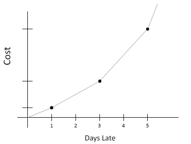
Late Cost as a Piecewise Linear Function

Let’s say that if a task is just one day late, there will be a small cost per day late (c₁). If a task is two or three days late, there will be a slightly larger cost per day late (c₂). If a task is four or five days late, the cost per day late will really increase (c₃) and if the task is more than five days late, the cost skyrockets (c₄). This results is a piecewise linear cost of lateness function that looks similar to this graph. Now the cost of ten tasks each a day late vs. the cost of one task that is ten days late is

c₁ * 10 tasks * 1 day vs. c₄ * 1 task * 10 days
10 * c₁ vs. 10 * c₄
where c₄ > c₁.

The CPLEX API has Piecewise Linear functionality (at least in versions 12.3 and 12.4) which I have tried and found works fine in general. It’s also fairly easy to write your own functionality using integer variables to indicate which category of lateness (0-1 day, 2-3 days, 4-5 days, 5+ days) each task falls into and multiplying these variables by the appropriate costs. I initially tried the CPLEX functionality for a large production model I was developing but I ran into edge cases that were behaving oddly so I did write my own constraints and did not see a performance difference, even with the largest datasets I used for testing.

Warning: As promised, Abstract Algebra joke ahead.

What is purple and commutes?
An abelian grape.
Thanks to my undergraduate Abstract Algebra teacher Dr. Todd Ashby for this joke. It is the only reason I still remember what abelian means.

User Experience and Optimization

As an Optimization Consultant, I spend most of my days working with clients and trying to build models and systems to meet their needs. In general, these are operational systems that run on command and the user sees the results without any human intervention. So they have to be robust to data and user input, which makes this much more difficult than one-off studies where you or I get to massage data and give the user what we want them to see.

An interesting side effect of this is that the models we build are only a portion of the overall system and can have minimal impact on the user experience. Partly this is because we spend a significant amount of time before the models ever go live with users making sure the results of the models make sense and are usable when the model team can still manually manipulate the data and output. But a significant portion of it is because when you are looking at an entire system you can’t focus on finding an error in a single piece of output. Therefore, most of the user experience is dictated by the UI.

On many optimization projects the UI is an afterthought and I think this is a grave miscalculation which threatens to undermine the entire project. The UI is the only interface a user has to see the model results, so it doesn’t matter if the model creates great suggestions and useful data if that doesn’t translate in a way that the user can see and utilize. I’ve seen good models derailed by a lacking UI as well as the effect a good UI can have on the usefulness of a model.

We like to think as OR experts that our models are all that really matter to the client, but in reality clients don’t care how fancy or simple our models are as long as the results they see make sense to them and are actionable. This is especially true as production models become more complex and the input data becomes larger and larger. Anybody else out there have similar results they’d like to share?

Additional Constraints Can Sometimes Help Performance

In linear and mixed integer programming, constraints often have a bad reputation. If a model is a family, then the constraints are the parents – making sure everyone does their homework, brushes their teeth, and in general obeys the rules. Parents can be a pain though, making us eat fruit when we want to eat candy and go to bed early when we want to stay up all night. And all of this parental guidance can hurt performance.

A modeler who has developed a large-scale MIP with many different types of constraints probably knows the anxiety that can accompany the addition of each constraint. Will this next constraint be the one that kills the model’s run time; the straw that breaks the model’s back? Even seemingly innocuous constraints can cause problems when added to an already complicated MIP. This can lead to a fear of adding a new constraint to a functioning model.

But just like good parents nurture their children and help them become more than they could be by themselves, constraints not only improve a model by adding realism to the model, they can even improve performance under certain circumstances. Let me give you an example that I ran into just last week while working on a large-scale MIP that already has 10-12 different types of constraints. One of these constraint types attempts to bring balance to the model by distributing a resource to a group of parties based on each party’s stake in the overall system. For instance, consider a long-term assignment problem where workers are assigned to shifts, including a limited number of prime shifts. To make sure the prime shifts are fairly distributed, workers with longer tenure in the company should receive more prime shifts.

Let p_i be the number of prime shifts that worker i has the right to based on his/her tenure and let s_ij equal 1 if prime shift j is assigned to worker i. Then let x_i be the cost (i.e. penalty) for not assigning enough prime shifts to worker i. The constraint to set x_i is then x_i≥p_i-∑_js_ij. If at least the “fair” amount of prime shifts have been assigned to worker i, then the penalty variable x_i has to be greater than or equal to 0. Otherwise, if worker i does not have enough prime shifts, the penalty variable x_i has to be greater than or equal to the gap between the fair number of prime shifts and the actual number of prime shifts. Adding x_i to the objective of minimizing the total cost of the schedule will guide the model towards a more fair schedule in terms of prime shift allocation since a more fair schedule will decrease the values of x_i‘s and thus the total cost of the model.

You will notice that in the constraint above, we’ve only set the minimum value of x_i. Since there is a cost associated with the value of this variable, the solver (in our case Cplex) should always choose the smallest value possible for the variable, thus providing the upper bound on the variable. But when we started to test the model after adding this constraint we realized that while it was obvious to us that the value of x_i should always be either zero or exactly equal to p_i-∑_js_ij, it was not so obvious to Cplex. The penalty variables were often set higher than “necessary” until the optimality gap got fairly small towards the end of the model solve. Now this in theory is not an issue since the optimal solution will always have the penalty variables set as low as they can be set. However, our model is large and has a 30 minute run time limit, so there may be times when the model run ends with a large optimality gap and thus those variables are set higher than necessary. Also, this adds to the complexity of the model and is one more thing Cplex has to try to optimize when, in fact, we know the exact value that each of these variables should be.

So we decided to try adding another constraint to provide the upper bound for these penalty variables (either zero or p_i-∑_js_ij depending on whether or not worker i has his/her fair number of shifts). The two constraints combine as x_i≥p_i-∑_js_ij and x_i≤p_i-∑_js_ij when p_i≥∑_js_ij; effectively x_i=p_i-∑_js_ij. Once we added this new constraint, Cplex is no longer able to set the value of the x_i‘s higher than “necessary”, reducing the search space. The solve starts with a lower optimality gap right away and the model solves faster.

In many cases, adding new constraints can negatively affect performance, but when the current set of constraints allow the solver more latitude than necessary, as in our case, adding a constraint or two to provide more guidance to the solver can improve performance and reduce run time. Sometimes having strict parents can be a good thing.

Ant Colony Optimization – Optimizing the Search for Food

When I saw that the latest Informs blogging challenge was OR and food, I immediately thought of the diet problem and minimizing grocery bills while maximizing nutrition (a knapsack problem, perhaps). But I also thought about Ant Colony Optimization which I have been interested in incorporating into my optimization toolbox for some time now. Ant Colony Optimization (ACO) is an optimization algorithm that at its very core is about food – finding the optimal path from an ant colony to a food source.

Ants are well-known in popular culture as being very strong (they can lift 20 times their weight — or a car if they were human!) but it is their food foraging skills that are the basis for ACO. An ant colony works together to efficiently find food sources, with scavengers laying pheromone paths to food sources that other ants in the colony can follow. As additional ants use this trail to successfully find food, they reinforce it. When a food source is exhausted, ants following the path will no longer find food and thus stop reinforcing the path, allowing it to expire. This allows ACOs to adapt to changes in the original problem without requiring a restart of the algorithm.

Ant Colony Optimization is similar to my all-time favorite metaheuristic, the Genetic Algorithm, since its optimization is based on biology (evolution in GAs vs. ant colony behavior in ACO) and it uses a population of entities (chromosomes and genes in GAs vs. ants in ACO) to find a solution. And like GAs, the solution representation is vital to the success of an ACO. There has to be a way to correlate an efficient path to food with a good solution in the original problem.

I am still in the introduction stage with Ant Colony Optimization and have not had a chance to code up an example problem to see the algorithm in action. But I have high hopes because I learned from Genetic Algorithms that Mother Nature is a pretty good optimizer. Hopefully in the next few weeks I’ll have time to put together a basic ACO algorithm and post a follow-up post comparing its performance with other optimization techniques. In particular, I have a few scheduling applications that are reduced to a set partitioning MIP currently solved with Cplex. I have been trying to development a GA as an alternative solution method but haven’t come up with an efficient chromosome representation for large-scale production problems. ACO has been used for a variety of problems, including set partitioning problems, so this is one of the first problems I will tackle.

Have you ever used Ant Colony Optimization and if so, what types of problems did it work well for? Do you have any “lessons learned” for Operations Researchers just getting started with ACO?

This blog post is a contribution to INFORMS’ monthly blog challenge. INFORMS will summarize the participating blogs at the end of the month.

My New Year Resolution – Take a Second Look

In thinking about new year resolutions and how I can improve my model building in 2012, I looked back on some of the ways I made big improvements to models I developed this past year. I spent the majority of my time working on a network distribution MIP that has a tight runtime SLA. As a result I have had to take a second, and even third or fourth, look at constraints I had already written to improve performance. Here are three ways I was able to improve my model that I will keep in mind while modeling this year:

1. The first way to formulate a constraint is not always the best. – Some constraints are very complex and it can be hard enough to formulate them a single way. But there are often alternatives which may not be as obvious or intuitive, but require less complexity or are easier to solve. This is a good time to brainstorm with your OR colleagues and expand your constraint toolkit.
2. Don’t use a bigger “Big M” than necessary. – When using the Big M method in constraints, it’s tempting to use a gigantic value for M to ensure that it dominates the constraint. But the value necessary to create the desired effect is often smaller than it might seem at first. I found that in some of my constraints it can be as small as 5000. For further reading Paul Rubin has a great blog post on this topic.
3. Re-examine the business requirement behind the constraint. – There was a particular tough constraint that, while easy to formulate, made the model very difficult to solve. When we reviewed the business requirement this constraint was meeting, we realized that a less restricted constraint formulation could still achieve the goal of the business requirement while not hurting model performance. We had over-restricted the problem unnecessarily. This is especially important to revisit later in the project, when you may have a better understanding of the business requirements than during the start of the project.

These are just a few ways to improve model performance that I’ll keep in mind this year as I am writing new models and refining existing models. I know there are many more ways to take a second look and improve existing models and I hope to try some more out this year. What are some ways that you have taken a second look and been able to reduce complexity and improve performance of a model?

This blog post is a contribution to INFORMS’ monthly blog challenge. INFORMS will summarize the participating blogs at the end of the month.

Optimizing Your Transportation Network can Reduce Your Carbon Footprint

In the past few years, I have worked on optimization models for different sectors of the Transportation industry that all have one thing in common: the goal always includes minimizing non-revenue trips, either explicitly defined as the objective function or captured as a cost to minimize. A non-revenue trip, sometimes called a ferry or deadhead, is a move to reposition resources at a new location. In a transportation scheduling or routing model, the majority (hopefully) of the moves yield a revenue: a commercial flight delivers paying customers to a destination, the post office delivers postage-paid mail to our homes, a delivery truck drops off the TV a customer purchased. These revenue trips require resources: airplanes, trucks, trains, pilots, drivers, fuel, etc… Non-revenue trips require the same resources but without generating the revenue required to pay for these resources. Regardless of the company and its products or services, unnecessary non-revenue trips are a waste of time, money, and resources.

An objective I have yet to see in any real-world optimization model I have worked on or encountered is to minimize the impact on the environment. That may be a little surprising since corporations are more focused on going green and helping the environment now than ever before. Recycling is common-place and my mother’s company even provides reduced fare for employees willing to take the bus to work rather than drive their own cars. While I am certain it is possible to include green objectives in a model, I haven’t had a client say “Minimize my emissions or my carbon footprint“. Or have I?

After all, an unnecessary non-revenue trip wastes more than time and money; most modes of transportation require non-renewable fossil fuels and produce emissions that are harmful to the environment. I do want to distinguish between unnecessary and necessary non-revenue trips. It’s generally impossible to eliminate non-revenue trips completely — sometimes a resource is needed in a location where none already exist. But often an optimization model can find ways to sequence stops to reduce the total number of non-revenue trips and minimize the distance of remaining non-revenue trips. Even just reducing non-revenue miles can save fuel and reduce emissions while saving the company money and time. Companies don’t need to explicitly model “green” objectives to help the environment.

Companies that utilize optimization to improve the efficiency of their operations should take an additional step and try to track the overall reduction in non-revenue trips and miles, and other areas of resource waste, as part of their effort to go green and become more environmentally friendly. A carbon footprint calculator like the one at Carbon Footprint can even help a company calculate the reduction in their carbon footprint as a direct result of their optimization efforts. Whether directly modeled in the objective or a by-product of other goals, companies can have a positive impact on the environment through the use of optimization and that benefits everyone.

This blog post is a contribution to INFORMS’ monthly blog challenge. INFORMS will summarize the participating blogs at the end of the month.

When the Data Changes Before the Model Even Finishes Solving

This month’s INFORMS blogging challenge topic is OR and analytics. Last Wednesday I was thinking seriously about this topic, in particular how OR and analytics, although separate fields, can benefit from each other, when I saw Michael Trick’s post outlining what each field can learn from the other. His analysis was very insightful and one of his points really hit home with me — #1 of what Operations Research can learn from Business Analytics:

It is not just the volume of data that is important:  it is the velocity.  There is new data every day/hour/minute/second, making the traditional OR approach of “get data, model, implement” hopelessly old-fashioned.  Adapting in a sophisticated way to changing data is part of the implementation.

Data volumes are increasing, data is coming from multiple sources in a variety of forms and states of completeness and cleanliness, and data is constantly changing. I am starting to see the effect ever-changing data can have on optimization more and more as my clients adapt the way they use our models . Many of our models are operational scheduling models that plan for a 24-48 hour planning horizon which generally starts a day or two in the future. The model sets the schedule for this future time period and was often designed to run only once a day. But when you plan this far in advance, things are bound to change. New tasks or assignments are added, existing ones are modified or may even be removed. How does this updated data affect the model’s results? Can it be incorporated into the current solution or is a completely new solution needed? What do we do when a model requires 30 minutes or an hour to solve but the data changes every minute? These needs are often not captured in the original business requirements for the optimization model but need to be addressed if the model is going to be effective in a real-time environment with volatile data.

Sometimes the model solves fast enough and schedules far enough in advance that it can be run continuously with data updates incorporated into each new solve. However this can result in solutions that change dramatically with each run which can be disruptive in a business environment. Consider a model that schedules workers for shifts. After the first run, a worker could be scheduled for a 8am shift. But after the next model run, the solution now has the worker scheduled for a 8pm shift. This is a pretty significant change. It also prevents the users from being able to notify the worker about his/her upcoming scheduled shifts because the schedule is constantly changing. One way that we have mitigated this problem is to place a higher value on the existing schedule in the objective function which prevents the optimization model from changing the current solution unless the change would result in substantial savings or benefits.

It may not be possible to continuously run an optimization model through a “full” solve because of a lengthy run time. One of our scheduling models essentially solves a set partition problem where the bulk of the model’s processing time is spent defining the feasible sets and only a fraction of the time is actually spent solving the optimization problem. In this case we need two modes: “full” mode and “update” mode. Full mode generates the entire space of feasible sets and then solves the resulting optimization problem. The model then switches to update model where it modifies, adds, and removes sets based on any data modifications that have occurred and solves the new optimization problem. These updates are significantly faster than regenerating all of the feasible sets so update mode runs in a fraction of the time that full mode requires.  We offset an initial long run-time with subsequent quick updates.

Finally, rather than attempting to retrofit an existing optimization model built to handle a static data set, we have started to assume that our models need to be capable of incorporating fluctuating data and design this into the models from the outset rather than wait for the client to ask for this ability down the road. It is much easier to design and build flexibility into an optimization model from the start than to try to add it at a later date. Our clients’ business needs are constantly evolving and we are working hard to anticipate their future needs and build Operations Research tools that evolve with them. We must adapt to the changing frontier of data: more data from multiple sources that changes frequently and often has not been “sanitized” for use in an optimization model.

Are you seeing an increased need to incorporate changing data into your Operations Research models, and if so, how are you handling this new and difficult requirement?

This blog post is a contribution to INFORMS’ monthly blog challenge. INFORMS will summarize the participating blogs at the end of the month.

Why is SpORts So Popular?

Several years ago I attended a SpORts (OR in Sports) session at the annual INFORMS meeting (I think it was New Orleans –> San Francisco 2005) and the room was packed. All the chairs were taken and latecomers resorted to standing against the back wall. Not only was this one of the most attended sessions of the conference (at least compared to the other sessions I attended), it also had an unusually high level of presenter-audience interaction.

In my experience it is fairly normal for a presenter to receive few, or even zero, comments and questions after a presentation. But in this SpORts session, several members of the audience interacted with the presenters; probing the data and methods, questioning the results and providing their own ideas for improvement. It made me wonder: What is it about OR applied to sports that made the audience so much more engaged than with other applications?

I think the answer lies in the accessibility of the data and results of a sports application of OR. Often only a handful of people know enough about an OR problem to be able to fully understand the problem’s data and judge the quality of potential solutions. For instance, in an airline’s crew scheduling problem, few people may be able to look at a sequence of flights and immediately realize the sequence won’t work because it exceeds the crew’s available duty hours or the plane’s fuel capacity. The group of people who do have this expertise are probably heavily involved in the airline industry. It’s unlikely that an outsider could come in and immediately understand the intricacies  of the problem and its solution.

But many people, of all ages and occupations, are sports fans. They are familiar with the rules of various sports, the teams that comprise a professional league, and the major players or superstars. This working knowledge of sports makes it easier to understand the data that would go into an optimization model as well as analyze the solutions it produces.

If I remember correctly, one of the presentations during that INFORMS SpORts session was about rating/ranking NFL quarterbacks. Professional football is one of the most popular sports in the United States and even those who aren’t a fan can probably name a NFL quarterback. And those that are fans probably have their own opinions about how good each quarterback is and how the various quarterbacks compare to each other. People not connected with the project are familiar with the basic data components and can even generate their own potential solutions and judge the solutions generated by others.

This fluency in the problem makes the methods and results more interesting to the audience because they can understand aspects of the algorithm and determine for themselves its efficacy. The audience doesn’t have to trust the authors that 5.6 is the optimal solution. And the results can even validate their own personal opinions (“I knew Peyton Manning was a better quarterback than Tom Brady!”). I am sure there are other reasons why sports is such a popular application of OR but regardless it is nice to see it generating enthusiasm and interest for OR.

This blog post is a contribution to INFORMS’ monthly blog challenge. INFORMS will summarize the participating blogs at the end of the month.